VALIDATION AND VERIFICATION IN COMPUTATIONAL FLUID DYNAMICS (CFD)

One method commonly used in design and research in fluid mechanics and heat transfer besides analytical and experimental is using a numerical method known as Computational Fluid Dynamics (CFD).

This method has been used for a long time to solve any engineering problems (fluid mechanics related) in many industries, from aerospace, maritime, automotive, manufacture, energy and renewable energy up to biomedical engineering.

Because this method is computer-based (no physical prototype needed), the total processes can be done quickly, flexible, low cost, deeper and more importantly no safety issues if the test is related to human interaction.

Nevertheless, some engineers and scientists are still skeptical about the accuracy of the CFD result because of the lack of operational CFD knowledge. (no matter how sophisticated your calculator is, if you hit the wrong input the output will be wrong right?). In this article, we will discuss the verification and validation of CFD method.

simulation of a centrifugal impeller using CFD (openFOAM software)

First, before we discuss verification and validation, we must understand some terminologies, these are (1) code, (2) simulation, and (3) Model:

(1) CODE: Is a bunch of computer instructions to gives input and definitions. This code has a strong relation to what software we used. Different software will have difference code characteristics.

(2) SIMULATION: Is the use of the model, in CFD case this is to obtain the results such as flow, pressure, velocity, etc. based on the input to the model.

(3) MODEL: Model is a representation of the physical system (in CFD case is the fluid flow or heat transfer) to predict the characteristics or output of the system. For example the geometrical size, inlet velocity, temperature in the wall, pressure at the outlet, etc. based on the physical system we want to mimic.

Credibility of a code, model and CFD simulation are obtained based on its uncertainty and error level. The value of uncertainty and error itself determines whether the program and computational method used are fitted with at least intuitively and mathematically or not. Then, validation determines whether the simulation is fitted with physical phenomena or not. Generally, validation used experimental methods if possible.

There are some disagreements among professionals about the standard procedure of verification and validation of CFD simulation. Although CFD is widely used, this method is relatively new. CFD is a complex method that involves non-linear differential equations to solve the theoretical equations or experimental equations in a discrete domain, in complex geometry. Hence, the error assessment for CFD is based on these tree root (1) theory, (2) Experiment, and (3) Computation.

USING THE CFD RESULTS
The accuracy level of CFD analysis depends on the use of the result itself. The conceptual design process doesn’t need an accurate simulation result, on the other hand, on the detail design process, we need accurate CFD results. Every quantity in CFD needs a different accuracy level, for example, we don’t need accurate temperature value in the design process of low-speed aircraft, but we need accurate temperature calculation when we are dealing with supersonic aircraft or rocket. In general, there are three categories of CFD simulation based on its accuracy demand: (1) Simulation for qualitative information, (2) Simulation to obtain incremental value, and (3) simulation to obtain the absolute value of a quantity.

(1) Simulation to obtain qualitative information
In this case, generally, experimental information data are hard or maybe too costly to obtain, so there’s no comparison data, and what engineers or scientists need is the “how it works” information, and how to optimize a flow without needing the exact value of each parameter. For example, a valve manufacturer wants to develop a novel design idea, and they want to prove the theory and see whether or not the flow is streamlined or chaotic in nature, they don’t need exact value of pressure drop, velocity, etc. in this conceptual design step: At least until they want to compare this design to an existing design (refer to category 2) and want to design the minimum thickness of this part before it is ready to manufacture (refer to category 3)

(2) Simulation to obtain incremental value
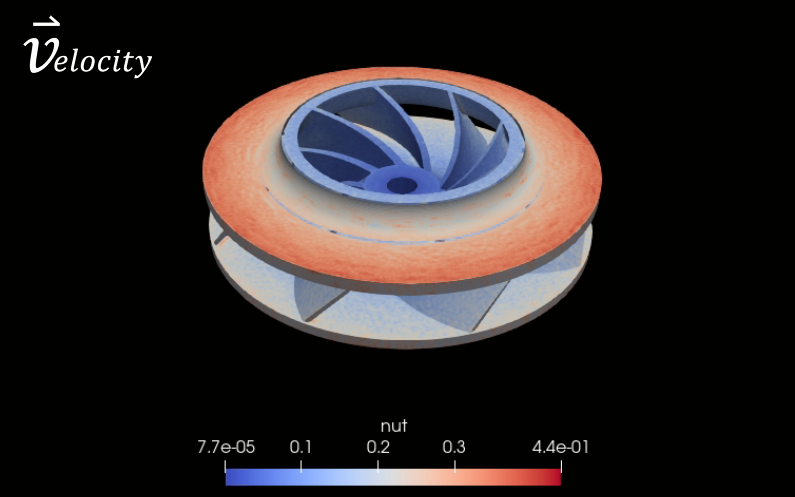
This scenario compares the incremental value with respect to some design or flows alteration with the same basic characteristics. For example, a company wants to modify an existing impeller blade in case of its blades number or its inlet angle (illustrates in the picture below). From this simulation, we could determine which impeller has the highest pressure difference regardless of its absolute pressure in the entire system. This type of simulation demands more accuracy than category 1.

(3) Simulation to obtain absolute quantity
This is the most accuracy-demanding simulation scenario and sometimes this simulation results are compared with the experimental result to validate the method, and the other results are used in the next design process such as calculating the L/D of an aircraft wing illustrates bellow:

FLOW CHARACTERISTICS
To conduct a model validation, we must understand the flow characteristic to get intuition whether the flow acts as expected physical phenomena or not. For example, if we simulate a projectile with the speed exceed the speed of sound, the shock wave phenomena should occur; or if we simulate flow in pipe in low Reynold number, the flow should be laminar, otherwise, it must be turbulent, and so on. This knowledge is important because CFD is only a “calculator” if we hit the wrong input, the output will be wrong, in fact, the settings in CFD software, in general, are varied and cause a headache if we don’t have this knowledge.

PHYSICAL MODEL
Physical model not only refers to the geometrical model, but these are also the following models to be considered in CFD simulation:

(1) Spacial dimension
Or the geometry (1D, 2D or 3D) of the object we want to model, sometimes this model is simplified with symmetry or reduces 3D into 2D to reduce the computational effort as long as it still represents the essence of the flow we want to analyze.

(2) Temporal dimension
This is a time dimension of the simulation we want to conduct. This is very important in transient simulation, but not significant if we want to simulate a steady simulation. For example, if we want to simulates an object that rotates 1 rotation/second, and we input the delta time 0,1 second, we will accommodate the 10 incremental motions in our simulation. But, if we input delta time 2 second, the computation will error because we can’t accommodate the “motion” of the object.

(3) Navier-Stokes Equation
This is the fundamental equation of fluid mechanics that models the flow velocity, pressure, gravity, viscosity and even rotational force in the flow.
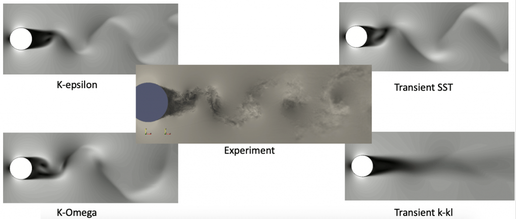
(4) Turbulent Model
This model is specially designed to model turbulent flow without calculating the whole (complex and computationally high effort) Navier-Stokes equation. The difference turbulent model we use will generate different results in our CFD simulation.

(5) Energy equation
Unlike classical solid mechanics, in fluid dynamics, energy generally refers to heat transfer and temperature change.

(6) Flow boundary condition
This is a mandatory input in our simulation. Boundary conditions input what flow characteristic we already have, for example, pressure in the inlet of a pipe (from a pump) or the velocity an aircraft during flight, etc.

CLOSURE
Even the setting in CFD simulation looks messy for CFD beginner, but a lot of scientists and engineers around the globe are publishing papers and journal continuously to share their setups and its accuracy compared to experimental as well as analytical results, hence CFD verification and validation becomes easier with these abundance references.

To read other articles, click here.

By Caesar Wiratama

aeroengineering.co.id is an online platform that provides engineering consulting with various solutions, from CAD drafting, animation, CFD, or FEA simulation which is the primary brand of CV. Markom.

TURBULENCE MODELS AND ITS USE IN COMPUTATIONAL FLUID DYNAMICS (CFD)

Fluid dynamics is a basic branch of physics and engineering, it’s usage is huge and varies, starts from rocket and aircraft design up to biomedical fluid analysis. Although this discipline has long developed and widely used, its mathematical formulations in fluid mechanics are not solved yet, such as the Navier-stokes equation, a non-linear partial differential equation.

Unlike solid mechanic laws such as Newton’s second law, F = m.a, or kinetic energy E = 1/2.m.v2, the Navier-Stokes equation not always solvable with an exact method using available mathematical tools. Even, a special prize is prepared for whoever solves this equation (Millenium prize). One reason that this equation is unsolvable is the random, unsteady and unpredictable flow characteristics in certain conditions, or known as turbulence.

To be exact, turbulence is a fluid flow condition with a random and chaotic characteristic that contains eddy, swirl, and flow instability. And the opposite of turbulence is laminar flow, the flow with a predictable pattern and with no disruption in its paths. In laminar flow, the Navier-Stokes equation easily solved, for example, becomes a well-known equation Bernoulli equation (Navier-Stokes equation in steady-state and negligible viscous effect). Because of its complexity to solve turbulence flow mathematically, a well-known scientist, Richard Feynman said that “turbulence is the most important and unresolvable problem in classical physics”.

Illustration of laminar and turbulent flow

Because no analytical mathematics method could solve this problem, scientists try to quantify this problem based on the experiment. One of the most popular ones is the work of Osborn Reynold (1883), which found a non-dimensional ratio that could predict whether the flow is turbulent or laminar, and its called Reynold Number. Mathematically, Reynold number, Re is the ratio between internal force and external force, or Re = rhoVL/miu, with rho = density, V = velocity, L = characteristic length and miu = fluid viscosity. With this Reynold number, we could predict for example the flow trough a pipe is laminar if Re<2300, turbulence if Re>4000 and transition if 2300<Re<4000, regardless of what fluid we are using and the diameter of the pipe. This value states that if internal force is dominated than external force the flow will turbulent and vice versa.

Even though we can predict the occurrence of turbulence, but we cant model the flow specifically at any certain point in an arbitrary geometry. Instead of solving the Navier-Stokes equation to get the solution of turbulence in each “streamline paths”, scientists and engineers try to groups each turbulence eddies and solve those eddies as a single mathematical object. A lot of methods were developed based on this idea, such as averaging the flow parameter in each eddy or solve a certain size of an eddy, and proper selection of turbulence model is a big deal in Computational Fluid Dynamics (CFD).

Unfortunately, there’s no instant answer which turbulence model must be used to a certain problem, the answer really depends to the detail of the problem, even same problem will need a difference turbulence model, for example, calculation of the lift-and-drag coefficient of an aircraft will have different best turbulence model selection for calculation of wall shear stress in the same aircraft and flow condition. But, you don’t have to worry about this situation, because nowadays, a lot of scientists and engineers publish their research about CFD and share their turbulence model usage compared to the other which is best suitable for their detail cases as our reference to our cases. Nevertheless, this article will discuss some well-known turbulence models and the rule of thumb of its selection.

DNS (DIRECT NUMERICAL SOLUTION)
DNS is a method of directly solving the Navier-Stokes equation in the fluid flow without assuming the turbulence as an average flow parameter. Although ideal in terms of physical significance, this method needs huge computational as well as hardware demand and not feasible in common engineering cases.

LES (LARGE EDDY SIMULATION)
The turbulent flow consists of eddies with certain scales, sometimes it dominated with small or large eddies, ranging from kilometers to microns. LES modeling used to well-determined eddy scale, usually small eddy. This method also needs a huge computational effort but more reasonable compared to DNS.

RANS (REYNOLD-AVERAGE NAVIER-STOKES)
This model uses the average value of turbulence fluctuating parameters. This model is widely used in common industrial problems because of its low computational effort compared to LES or DNS even its accuracy is lower.

DES (DETACHED EDDY SIMULATION)
This turbulence model is the combination of LES and RANS, which solves near boundary layer region using RANS, and far boundary layer using LES. The picture below illustrates the DES concept.

Illustration of DES idea

In the region near boundary layer, velocity gradient becomes considerably high and determines the shear stress in the wall as well as turbulence boundary layer characteristics, to accommodate this situation, extremely small mesh must be used near the boundary layer, but this is sometimes not feasible in terms of computational effort and time, hence the wall-function is often used to modify velocity distribution in the boundary layer without considering extremely small mesh.

These are the commonly used turbulence models in the commercial as well as opensource CFD software and its rule of thumbs:

Spalart-Allmaras

  • One equation
  • No wall function
  • Stable and easy to convergent
  • Advantages: Aerodynamics flow and transonic regime
  • Limitation : Not accurate for shear flow, separated flow and decaying turbulence

K-Epsilon

  • Two equations
  • Has wall function
  • Easy to convergent and need relatively small memory
  • Advantages: Free stream flow
  • Limitation: Not accurate for no-slip wall, adverse pressure gradient, high curvature, and jet flow

K-Omega

  • Two equations
  • Omega is easier to solve than epsilon
  • Has wall function
  • Easy to convergent and need relatively small memory
  • Advantages: Internal flow, high curvature, separation, and jet flow

K-Omega SST (SHEAR STRESS TRANSPORT)

  • Two equations
  • Has wall function
  • Combination of k-epsilon for free stream flow and k-omega for near boundary layer flow
  • Advantage: Separation and jet flow
  • Limitation: Hard to convergence

LES Smargorinsky & Spalart-Allmaras

  • Solves eddies flow in certain size/scale
  • Separates small and large eddies
  • Advantages: Thermal fatigue, vibration, buoyant flows
  • Limitation: Hard to capture near-wall flow

To read other articles, click here.

By Caesar Wiratama

aeroengineering.co.id is an online platform that provides engineering consulting with various solutions, from CAD drafting, animation, CFD, or FEA simulation which is the primary brand of CV. Markom.

THE FLUID CONSERVATION OF MASS EQUATION

The conservation of mass is one of three basic fluid fundamental laws (or general physical laws actually). This principle actually is quite simple to understand, a person doesn’t need to become a fluid engineer to calculate the mixture total weight of 100 grams of coffee mixed with 200 grams of milk, it simply becomes 300 grams of coffee milk.

This law not only governs the fluid flow problems, but it also can be applied to a chemical formula such as the mass balance of oxygen and hydrogen reacted to become water. 32 kg of oxygen reacts with 4 kg of hydrogen will form 36 kg of water.

This law is very universal in nature, we can apply this mass conservation law for every engineering problem in the earth as well as anywhere in the universe. The only exception for this law is Einstein’s mass and energy equation E = m.c2, which states that mass can be converted into energy when the mass is “disappear”, but this condition rarely happen in fluid dynamic problems, and only relevant for most nuclear reactions and near the speed of light physics problems. So, we can ignore this relation in our following discussion.

In fluid mechanics problems, sometimes it is not useful to determine the amount of mass of the fluid, imagine if you should measure the total mass inside a long pipe, or maybe the total of air comes out from an air conditioner system: it will become a tedious activity and not feasible with our measurement devices. To better formulate this mass conservation law, in fluid mechanics, we often used the rate of change of the mass or known as mass flow rate, defined as the amount of mass divided by the time.

mass flow rate = total mass / total time

In this form, the conservation of mass law sometimes called the continuity principle. For example, one could easily measure the mass flow rate of flow through a pipe in kg/s or maybe kg/hour with a flow measurement device without having to know the total amount of mass along the pipe.

From this mass flow rate idea, the fluid conservation of mass can be defined as total mass flow rate comes in a control volume will be equal to mass flow rate comes out a control volume plus the mass increasing/decreasing rate inside the control volume, or mathematically:

mass flow rate in = mass flow rate out + rate of mass change in the system

Imagine if we have a bath up with water tap opens and flow with mass flow rate 1 kg/s, then we open the bottom drain causes the flow out about 0,8 kg/s, we will find our bath up will fill with water in 0,2 kg/s rate. Quite simple right?

In an internal flow such as pipes or tubes, the mass flow rate can be calculated using the following equation:

mass flow rate = density*area*velocity

Another important concept of mass conservation law is the volume flow rate or simply flow rate. This is a very useful concept if we want to analyze an incompressible flow such as water, oil, or air at low-speed operation. (Incompressible flow is a flow with negligible density change with respect to pressure, temperature, time, etc.). The volume flow rate mathematically described as:

Volume flow rate = area*velocity

If we consider a steady-state flow (rate of mass change inside control volume = 0), we can rearrange the conservation of mass equation in the form of volume flow rate as:

area 1 * velocity 1 = area 2 * velocity 2

The above equation is a very important relationship between area and velocity in incompressible flow, it simply states that if we decrease the area, we will increase the velocity or vice versa.

velocity distribution in a ventury device using CFD

From the above picture, we can see the flow of fluid inside a ventury device. The flow inlet is on the left and flows in the right direction. We can see low-speed flow at the inlet (colored blue) then become faster (colored red) at the center of the ventury as the cross-sectional area decreases. Then, the flow velocity gradually becomes slower as the cross-sectional area grows streamwise.

The same principle we often use in our daily life is reducing the water hose outlet with our thumb to increase the velocity (hence increase the range of water) is actually the application of continuity principle.

Another example of this area to velocity relationship is the principle of airfoil’s aerodynamic shows below:

velocity distribution around NACA 2412 airfoil using CFD

It can be seen that airflow velocity above the airfoil faster than under the airfoil. for the kinematics point of view, the curve-shape of the top airfoil surface creates a longer path for flow to reach the airfoil end, hence with the same given time will need a higher velocity.

Flow around airfoil velocity changes based on its location

Then, if we want to explain the above phenomena using a continuity point of view, we can make an imaginary line above the airfoil, then compare the “cross-sectional area” of the flow. We can see at the beginning (point 1), the velocity is similar to free stream velocity, then at the top part of the airfoil (point 2) cross-sectional area reduces, hence increase the velocity on the top of the curve, finally at point 3, velocity goes back to free stream velocity as the “cross-sectional” area back to its original size.

To read other articles, click here.

By Caesar Wiratama

aeroengineering.co.id is an online platform that provides engineering consulting with various solutions, from CAD drafting, animation, CFD, or FEA simulation which is the primary brand of CV. Markom.

Boiler dengan bahan bakar batu bara

Desain pompa, kompresor, dan fan (turbomachineries) menggunakan CFD

Computational fluid dynamics (CFD) adalah metode numerik untuk menyelesaikan permasalahan-permasalahan dinamika fluida menggunakan bantuan komputer. Metode ini sudah cukup lama digunakan oleh para engineer pada berbagai ranah industri seperti aerospace, otomotif, proses, energi, bahkan hingga medis. Salah satu industri yang didominasi oleh penggunaan CFD ini adalah desain turbomachinery seperti pompa, turbin, kompresor, fan dan blower.

Turbomachinery pada dasarnya adalah mesin yang mentransfer energi antara fluida dan rotor. Untuk fan, blower dan kompresor, energi mekanik dari putaran rotor (yang digerakkan oleh motor listrik atau bahan bakar) akan menggerakkan fluida yang ada di sekitarnya sehingga menghasilkan kecepatan aliran yang tinggi (untuk blower dan fan) atau meningkatkan energi fluida dalam bentuk tekanan yang tinggi yang disertai kenaikan temperatur (untuk kompresor). Sedangkan pompa biasanya mengacu pada sistem penambah tekanan fluida yang incompressible seperti air atau bahan kimia.

Kemudian turbin bekerja sebaliknya, fluida yang mengalir membawa energi berupa kecepatan, tekanan atau terkadang temperatur (entalpi) mendorong turbin hingga berputar dan menghasilkan energi mekanik yang dimanfaatkan untuk menghasilkan listrik dengan memutar generator atau dimanfaatkan untuk memutar kembali fan, blower atau kompresor yang dihubungkan dengan poros.

contoh turbomachinery dalam mesin pesawat terbang (terdapat fan, kompresor dan turbin dalam satu sistem)

CFD memegang peranan yang sangat penting dalam desain turbomachinery, keunggulan utamanya adalah mengurangi siklus desain dalam meningkatkan performa, mengurangi berat dan biaya. sebagai contoh, gambar dibawah ini mengilustrasikan variasi sudut blade saat masuk kompresor dan jumlah blade pada kompresor sentrifugal. Menggunakan bantuan komputer, kita dapat dengan sangat cepat dan mudah mengedit model tersebut kemudian langsung disimulasikan menggunakan CFD dan dalam waktu singkat memperoleh prediksi performa yang kita inginkan. Bayangkan ketika kita harus “mengedit” model tersebut secara fisik, mungkin akan memakan cukup banyak waktu dan biaya untuk membuat satu model saja.

Ilustrasi modifikasi blade kompresor sentrifugal menggunakan komputer

Salah satu fitur yang cukup penting yang dimiliki oleh CFD adalah kemampuanya untuk melihat secara detail parameter-parameter aliran (kecepatan, tekanan, temperatur dll) disetiap lokasi dan di setiap waktu untuk analisis transient. Kita dapat dengan sangat mudah “menunjuk” lokasi tersebut untuk dianalisis tanpa harus menginstal probe atau sejenisnya, dan kita dapat melakukan “zoom” dalam dimensi waktu dengan mengatur step waktu yang kita inginkan tanpa harus menggunakan kamera super cepat.

detail distribusi tekanan hasil CFD

Selain analisis aliran fluida, CFD juga sangat memegang peranan penting dalam desain turbomachinery karena kapabilitasnya dalam analisis perpindahan kalor. Berikut adalah contoh distribusi temperatur pada rotor turbin uap pada saat proses pendinginan dan distribusi .

distribusi temperatur pada rotor turbin uap dengan CFD

Pada era yang sudah serba canggih dan cepat ini, teknologi komputasi paralel memungkinkan perhitungan yang jauh lebih cepat dibantu dengan high performance computer yang menyokong kemampuan CFD ini. Analisis CFD untuk desain turbin pada umumnya menggunakan software komersial seperti ANSYS FLUENT atau software opensource seperti openFOAM.

Menggunakan CFD, prediksi peningkatan entropi saat terjadinya vortices dan wake mix pada aliran transient dapat diprediksi dengan sangat mudah, bahkan saat ini yang menjadi hambatan adalah justru validasi hasil CFD tersebut karena sulitnya perancangan metode eksperimen untuk kasus ini.

Berikut adalah contoh-contoh kasus simulasi CFD turbomachinery:

Salah satu hal yang cukup menarik dari metode komputasi ini adalah kemampuanya untuk saling terkoneksi dengan metode analisis lain. Seperti misalkan kemampuan untuk mengeksport hasil simulasi aliran dari CFD sebagai input tekanan pada permukaan blade untuk simulasi struktural. Berikut adalah contoh simulasi struktural (FEA) yang inputnya menggunakan hasil simulasi CFD:

Analisis flutter menggunakan modal analysis yang dipadukan dengan hasil CFD
Analisis tegangan pada sambungan blade dengan beban mekanik serta fluida hasil simulasi CFD

By Caesar Wiratama

aeroengineering services merupakan jasa layanan dibawah CV. Markom dengan berbagai jenis solusi, mulai dari drafting CAD, pembuatan animasi, simulasi aliran dengan CFD dan simulasi struktur dengan FEA.

RISET DESAIN TURBIN ANGIN DAN TURBIN AIR DENGAN CFD

Desain turbin angin maupun turbin air telah banyak dibahas dalam buku-buku teori mekanika fluida, baik performanya maupun karakteristik aliran fluidanya. Dalam referensi-referensi tersebut banyak disediakan persamaan-persamaan untuk menentukan hubungan antar-parameter seperti efisiensi, daya, torsi, energi potensial dari fluida serta hubunganya dengan efisiensi turbin.

Namun, prediksi dari parameter-parameter tersebut kadang kala terdapat variabel-variabel yang tidak dapat dihitung secara analitis, misalkan saja koefisien daya atau torsi yang dihasilkan pada rpm dan kecepatan fluida tertentu karena adanya interaksi fluida 3D yang kompleks serta pola-pola aliran yang tidak ideal, seperti turbulensi, vortex dan interaksi antara turbin dengan komponen sekunder lainya. Parameter-parameter tersebut secara umum dihitung menggunakan data-data empiris dari uji laboratorium baik menggunakan wind tunnel, water tunnel maupun uji lapangan langsung yang cukup memakan waktu dan biaya karena fleksibilitasnya yang rendah.

Salah satu metode yang cukup populer, yang memadukan antara perhitungan teori analitis dengan eksperimen adalah menggunakan eksperimen numerik yang dalam kasus mekanika fluida dikenal dengan istilah Computational Fluid Dynamics (CFD). Metode ini memodelkan turbin secara 3D menggunakan komputer, kemudian model tersebut disimulasikan terhadap aliran fluida yang ada di sekitaranya, sehingga dapat diperoleh solusi-solusi seperti torsi, daya dan efisiensi secara lebih komprehensif karena mempertimbangkan pola aliran 3D maupun interaksi-interaksi dengan komponen-komponen sekitarnya yang dapat mempengaruhi aliran.

Dewasa ini, metode CFD sudah sangatlah berkembang, sehingga perhitungan aliran-aliran turbulen yang kompleks dapat dimodelkan dengan cukup akurat, bahkan aliran dua fasa yang terjadi misalkan pada turbin air vortex maupun cross flow dapat dimodelkan secara real tanpa penyederhanaan perhitungan satu fasa.

Berikut adalah contoh-contoh project turbin yang pernah kami kerjakan:

simulasi HAWT dengan CFD
simulasi VAWT dengan CFD
Aliran dua fasa (air dan udara) pada turbin air cross flow
Pola aliran free surface pada gravitational vortex water turbine
Distribusi tekanan pada permukaan turbin kaplan
pola distribusi streamline pada turbin kaplan

Dengan simulasi-simulasi yang dilakukan diatas, kita dapat dengan mudah membandingkan konfigurasi-konfigurasi turbin yang ada dengan sangat fleksibel. Berikut adalah contoh grafik koefisien daya terhadap TSR untuk dua turbin angin VAWT yang divariasikan kontur permukaanya:

Nilai dari koefisien daya (Cp) seperti contoh diatas tidak dapat diperoleh dengan mudah menggunakan metode analitis, terutama jika kita ingin membuat inovasi-inovasi terbaru yang belum pernah ada data eksperimental sebelumnya

By Caesar Wiratama

aeroengineering services merupakan jasa layanan dibawah CV. Markom dengan berbagai jenis solusi, mulai dari drafting CAD, pembuatan animasi, simulasi aliran dengan CFD dan simulasi struktur dengan FEA.

RISET AERODINAMIKA PESAWAT TERBANG DENGAN CFD

Desain pesawat terbang merupakan suatu kegiatan yang cukup menantang dan menjadi passion bagi sebagian orang. Dalam tahap desainya, pesawat terbang terdiri dari proses-proses yang cukup panjang seperti conceptual design, preliminary design, detail design hingga desain untuk proses produksinya.

Cukup banyak terdapat buku-buku terkait dasar-dasar desain aerodinamika pesawat terbang, mulai dari teori pemilihan airfoil, penentuan ukuran sayap (span, chord, twist dll) hingga teori tentang interaksi antar komponen misalkan interaksi antara aliran propeller dengan sayap, interaksi fuselage dengan sayap, interaksi sayap dengan empenage dan lain sebagainya. Namun, teori-teori tersebut sangatlah umum dan kadang membutuhkan ketelitian dan pekerjaan yang ekstra untuk memperoleh konfigurasi yang optimal dari semua interaksi-interaksi tersebut.

Terlebih lagi, untuk pesawat dengan sayap non konvensional seperti adanya winglet, swept-back, sayap delta, ataupun dengan twist tertentu, teori-teori yang sudah ada kadang tidak cukup untuk mendeskripsikan permasalahan-permasalahan tersebut.

Di sisi lain, untuk mendapatkan analisa yang lebih komprehensif seperti aerodinamika karena interaksi-interaksi yang telah dijelaskan diatas serta konfigurasi-konfigurasi yang unik biasa digunakan metode eksperimen menggunakan wind tunnel. Metode ini cukup baik dalam menghasilkan data yang akurat, namun cenderung tidak fleksibel karena kita harus membuat model fisiknya terlebih dahulu yang mana membutuhkan waktu dan biaya.

Salah satu metode yang sudah berkembang dengan cukup cepat sebagai pertengahan antara metode analitis dengan eksperimen adalah menggunakan computational fluid dynamics (CFD). Metode yang sudah digunakan oleh NASA sejak tahun 1970an untuk mendesain pesawat supersonik tersebut mampu merepresentasikan model pesawat terbang secara keseluruhan tanpa penyederhanaan fitur-fitur utamanya sehingga mampu memprediksi performa aerodinamika secara lebih komprehensif. Kemudian, metode CFD ini sangatlah fleksibel dibandingkan dengan eksperimental, karena model yang harus kita buat hanyalah model virtual yang dibuat menggunakan komputer. Metode ini sering kali disebut juga dengan eksperimen numerik.

simulasi CFD pada pesawat tempur dengan CFD openFOAM

Meskipun riset menggunakan CFD dapat dilakukan secara independent, yaitu tidak perlu dibandingkan dengan data eksperimen (bahkan desain peralatan uji laboratorium sering kali didesain menggunakan metode CFD ini), tidak jarang juga hasil CFD dibandingkan dengan eksperimen lab. Sebagai contoh hasil uji CFD winglet pesawat boeing 737 yang kami bandingkan dengan hasil uji wind tunnel di laboratorium yang kami bandingkan nilai L/D nya terhadap sudut serang sebagai berikut:

Dari hasil perbandingan di atas, dapat dilihat hasil yang diperoleh dari simulasi CFD dan eksperimen wind tunnel memiliki trend dan nilai yang berdekatan. Dapat dilihat pula bahwa simulasi CFD mampu memprediksi aliran stall yang terjadi tidak seprti perhitungan analitis yang hanya terbatas pada aliran sebelum stall.

Selain perhitungan-perhitungan dasar seperti gaya angkat, drag, moment, lift-to-drag ratio dll, dapat juga dianalisis bagian-bagian lain yang cukup detail seperti aliran pada landing gear, aliran sekitar engine UAV, atau aliran stall dan vortex, serta desain control surfaces sebagai contoh:

simulasi stall pada airfoil dengan CFD openFOAM
simulasi tip vortex dengan CFD openFOAM
desain flap dengan CFD openFOAM

Selain memprediksi karakteristik aerodinamika pada aliran diluar pesawat, CFD juga dapat digunakan untuk menganalisis reaksi kimia seperti pembakaran pada ruang bakar (combustion chamber) mesin pesawat terbang sebagai berikut:

simulasi pembakaran pada turbin gas propulsi dengan CFD openFOAM

Meskipun memiliki kapabilitas dan hasil yang cukup detail dan komprehensif, namun bagi operator yang belum terbiasa menggunakan CFD dapat menjadi kesulitan tersendiri dalam mempelajari nya. Kami memberikan solusi berupa project support serta konsultasi simulasi pada pesawat terbang.

>> KLIK DI SINI UNTUK JASA SIMULASI CFD PESAWAT TERBANG !

By Caesar Wiratama

aeroengineering services merupakan layanan dibawah CV. Markom dengan solusi terutama CFD/FEA.