Momentum Analysis of fluid flow

In fluid mechanics, we are dealing with highly “squishy” material, unlike solid material which is easily modeled using relatively simple mathematical relationships. The nature of fluid flow complexity makes the “higher-order” mathematical modeling of fluid flow to get a detailed problem description such as the Navier-stokes equation by utilizing the differential equation approach or alternatively using the empirical method.

But, in engineering practice, sometimes we don’t even need a detailed problem description just to obtain some simple parameters. The simpler way to model this condition is by using the control volume method to estimate the result, in this case, momentum calculation.

Talk about momentum, the best way to describe it is by using the Newton’s law, mathematically described as:

F = m.a = d(m.v)/dt

With F = force, m = mass, a = acceleration, v = velocity, t = time. Then, the product of mass and velocity, m.v is also called linear momentum, hence the equation above can also be read as force is equal to the rate of change of linear momentum. Remember the force, velocity and momentum are vector quantity, so we must treat each equation for each direction (x,y,z).

Back to fluid flow problem, consider water flow in a pipe then accelerated trough a hose then the water sprayed to the atmospheric condition. To calculate the reaction force generated by the momentum change of the water, first we must consider the control volume to focus our analysis:

To analyze the problem, we must define the general momentum law of fluid flow in the control volume (CV) as:

The sum of all external forces acting on a CV = The time rate of change of the linear momentum of the contents of the CV + The net flow rate of linear momentum out of the control surface by mass flow

With body force usually a gravity force and surface forces usually pressure, viscous and other forces. The first term of the right hand side of the equation is transient term, if the flow is steady (time independent), and the equation is simply become:

total F = total (B.mdot.v)out – total (B.mdot.v)in

with mdot = mass flow rate and B is the momentum-flux correction factor, with B = 1 for the case of uniform flow over an inlet and outlet. Back to our water hose problem, consider the mass flow rate of the water is 2 kg/s with flow enter the control volume (from the pipe) is 1 m/s, then accelerated after pass trough the reducing nozzle (read continuity) the speed become 5 m/s. Using the above equation, we can calculate the total F acting to the CV as (assume B = 1)

total F = 2*5 – 2*1 = 8 Newton

The total force is 8 Newton in the direction of outlet velocity (because positive result). In the outlet velocity direction? yes, right, we just calculated the action force, then the reaction force acted to the CV will be in the opposite direction (third Newton’s law).

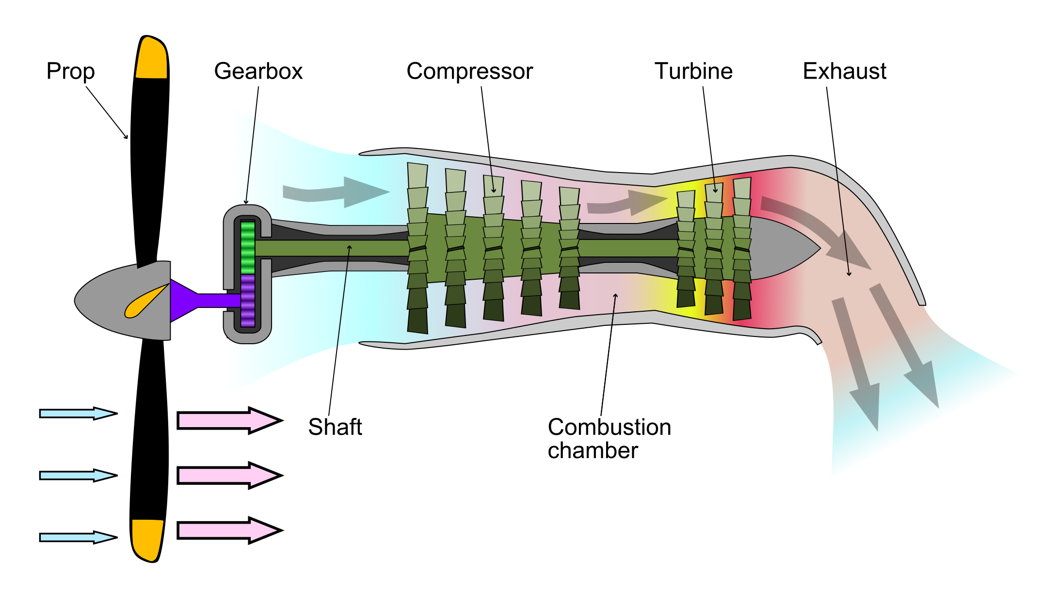
This method is quite simple and fast compared to the differential analysis with a lot of simplification of course. We can also calculate more “complex” problem such as rocket reaction force or aircraft jet without any complex mathematical modelling for estimating the result.

To learn more about a more detailed fluid flow problem, you can read about the Navier-Stokes equation and Computational Fluid Dynamics (CFD) method for the numerical method to solve the complex differential equation by utilizing computer power.

Water hose simulation using computational fluid dynamics

To read other articles, click here.

By Caesar Wiratama

aeroengineering.co.id is an online platform that provides engineering consulting with various solutions, from CAD drafting, animation, CFD, or FEA simulation which is the primary brand of CV. Markom.

THE BERNOULLI EQUATION

Using existing laws of nature, people could utilize those principles to develop engineering systems that changed the world. In fluid mechanics, one of the equations that really phenomenal because of its simplicity and tremendous usage is the Bernoulli equation.

There are three universal laws of the universe, (1) mass conservation, (2) momentum conservation, and (3) energy conservation. In solid mechanics, the momentum equation is described using Newton’s second law, F = m.a, similarly, in fluid mechanics, this law is described using Bernoulli equation (In fact, the most general and comprehensive mathematical expressions of momentum conservation is Navier-Stokes equation, but, it is very complicated mathematically).

To understand this principle, let’s make the mathematical formalization using this free body diagram:

Using well known mechanical energy conversion equation, the total of kinetic energy and potential energy will always be the same everywhere. Mathematically describes as follow:

With m = mass, g = gravitational acceleration, v = velocity, and H = height. In fluid mechanics, “energy” can be added by utilizing a pump to add pressure or sucks pipe outlet, hence the “pressure energy” term, E = p.V should be added on both sides of the equation.

with p = pressure, and V = volume. Then, we should realize that it is a tedious task or even impossible to calculate the whole mass and volume inside the pipe, what should we do is divide both sides with Volume so we can get:

with rho = is the fluid density. This equation is basically the well known Bernoulli equation. This equation is quite useful because it could predict the relationship between velocity and pressure. The following equation is for incompressible flow (constant density such as water), and negligible heigh difference. you can see how simple is this equation:

VENTURI TUBE AND EJECTOR

The above relationship is quite interesting, it is an inverse relationship between pressure and the square of velocity, it means if we have more velocity, the pressure will drop. Let’s discuss a venturi tube:

From the continuity equation (read here), we know that if we reduce the flow cross-sectional area, the velocity will be greater (as can be seen red-colored zone at the center), hence the pressure will be drop as the velocity increase quadratically. This pressure reduction can be calculated to measure the flow velocity, this is how venturi meter basically works.

The machine that has an identical principle as a venturi tube is the ejector. This device ejecting high-speed fluid through a nozzle and creates local negative pressure, this negative pressure sucks fluid from the neutral pressure chamber then push it to create flow. This is commonly used in industrial process applications:

AIRFOIL PRINCIPLE

Another example of this lift generation in an Airfoil as follows:

Imagine two particles flow from the leading edge (front of airfoil), one follows the top (curved) path and another follows the bottom (less curved) path, those particles will meet in the trailing edge at the same time, the curved path has longer traveling distance hence the velocity should be higher (This explanation is not proper for advance aerodynamics discussion, but good enough to understand this basic principle). Because of the higher velocity (colored red) at the top surface, the pressure expected to drop, hence creating suction to pull the airfoil upward (lift force).

This velocity and pressure relationship often causes a misunderstanding. If the flow velocity increase causes the pressure reduction, why if we shoot away higher-velocity water to our body the “pressure” we feel is greater? This statement is not totally wrong, but we must look closer in the flow region really close to our body, when the flow hits our body, the velocity in that local area suddenly became near zero in the normal direction to our body and deflected to the side, and as you can expect, the pressure has become higher significantly. This near-zero velocity region when the flow is hitting is called stagnation point.

TORICELLI THEOREM

The other interesting case of Bernoulli equation is the Toricelli theorem, see the free body diagram below:

The top tank and bottom tank are exposed to atmospheric pressure, hence P1 = P1. Then, the diameter of the top tank much larger than the bottom hole, so we can assume that V1>>V2, or V2 ~ 0. Then, consider H = H1-H2, we can rearrange the Bernoulli equation become:

This is a very simple and elegant equation to predict the flow velocity in the bottom of a tank with a hole versus its fluid height.

LIMITATIONS

And much more we can explore with the Bernoulli equation. Despite its usefulness, this equation, of course, has some limitations as follow:

  1. The flow is steady, there is no change in flow with respect to time.
  2. Inviscid flow, there is no viscosity (the tendency of the fluid to “sticking” to each other or to the solid wall) taking into account in this equation. The modeling of viscosity is accommodated in the Navier-Stokes equation.
  3. There is no shaft or fan power inside the flow.
  4. Incompressible flow, flow with thermal expansion effect can be analyzed using more comprehensive closure such as ideal gas equation or enthalpy equation in thermodynamics.
  5. There’s no heat and mass transfer
  6. The flow is along a streamline, no disruption of flow, no branches or turbulent flow.

To read other articles, click here.

By Caesar Wiratama

aeroengineering.co.id is an online platform that provides engineering consulting with various solutions, from CAD drafting, animation, CFD, or FEA simulation which is the primary brand of CV. Markom.

THE FLUID CONSERVATION OF MASS EQUATION

The conservation of mass is one of three basic fluid fundamental laws (or general physical laws actually). This principle actually is quite simple to understand, a person doesn’t need to become a fluid engineer to calculate the mixture total weight of 100 grams of coffee mixed with 200 grams of milk, it simply becomes 300 grams of coffee milk.

This law not only governs the fluid flow problems, but it also can be applied to a chemical formula such as the mass balance of oxygen and hydrogen reacted to become water. 32 kg of oxygen reacts with 4 kg of hydrogen will form 36 kg of water.

This law is very universal in nature, we can apply this mass conservation law for every engineering problem in the earth as well as anywhere in the universe. The only exception for this law is Einstein’s mass and energy equation E = m.c2, which states that mass can be converted into energy when the mass is “disappear”, but this condition rarely happen in fluid dynamic problems, and only relevant for most nuclear reactions and near the speed of light physics problems. So, we can ignore this relation in our following discussion.

In fluid mechanics problems, sometimes it is not useful to determine the amount of mass of the fluid, imagine if you should measure the total mass inside a long pipe, or maybe the total of air comes out from an air conditioner system: it will become a tedious activity and not feasible with our measurement devices. To better formulate this mass conservation law, in fluid mechanics, we often used the rate of change of the mass or known as mass flow rate, defined as the amount of mass divided by the time.

mass flow rate = total mass / total time

In this form, the conservation of mass law sometimes called the continuity principle. For example, one could easily measure the mass flow rate of flow through a pipe in kg/s or maybe kg/hour with a flow measurement device without having to know the total amount of mass along the pipe.

From this mass flow rate idea, the fluid conservation of mass can be defined as total mass flow rate comes in a control volume will be equal to mass flow rate comes out a control volume plus the mass increasing/decreasing rate inside the control volume, or mathematically:

mass flow rate in = mass flow rate out + rate of mass change in the system

Imagine if we have a bath up with water tap opens and flow with mass flow rate 1 kg/s, then we open the bottom drain causes the flow out about 0,8 kg/s, we will find our bath up will fill with water in 0,2 kg/s rate. Quite simple right?

In an internal flow such as pipes or tubes, the mass flow rate can be calculated using the following equation:

mass flow rate = density*area*velocity

Another important concept of mass conservation law is the volume flow rate or simply flow rate. This is a very useful concept if we want to analyze an incompressible flow such as water, oil, or air at low-speed operation. (Incompressible flow is a flow with negligible density change with respect to pressure, temperature, time, etc.). The volume flow rate mathematically described as:

Volume flow rate = area*velocity

If we consider a steady-state flow (rate of mass change inside control volume = 0), we can rearrange the conservation of mass equation in the form of volume flow rate as:

area 1 * velocity 1 = area 2 * velocity 2

The above equation is a very important relationship between area and velocity in incompressible flow, it simply states that if we decrease the area, we will increase the velocity or vice versa.

velocity distribution in a ventury device using CFD

From the above picture, we can see the flow of fluid inside a ventury device. The flow inlet is on the left and flows in the right direction. We can see low-speed flow at the inlet (colored blue) then become faster (colored red) at the center of the ventury as the cross-sectional area decreases. Then, the flow velocity gradually becomes slower as the cross-sectional area grows streamwise.

The same principle we often use in our daily life is reducing the water hose outlet with our thumb to increase the velocity (hence increase the range of water) is actually the application of continuity principle.

Another example of this area to velocity relationship is the principle of airfoil’s aerodynamic shows below:

velocity distribution around NACA 2412 airfoil using CFD

It can be seen that airflow velocity above the airfoil faster than under the airfoil. for the kinematics point of view, the curve-shape of the top airfoil surface creates a longer path for flow to reach the airfoil end, hence with the same given time will need a higher velocity.

Flow around airfoil velocity changes based on its location

Then, if we want to explain the above phenomena using a continuity point of view, we can make an imaginary line above the airfoil, then compare the “cross-sectional area” of the flow. We can see at the beginning (point 1), the velocity is similar to free stream velocity, then at the top part of the airfoil (point 2) cross-sectional area reduces, hence increase the velocity on the top of the curve, finally at point 3, velocity goes back to free stream velocity as the “cross-sectional” area back to its original size.

To read other articles, click here.

By Caesar Wiratama

aeroengineering.co.id is an online platform that provides engineering consulting with various solutions, from CAD drafting, animation, CFD, or FEA simulation which is the primary brand of CV. Markom.

COMPUTATIONAL FLUID DYNAMICS AND NAVIER-STOKES EQUATION

What was first imagined in your mind when you hear the word CFD? Some people sometimes imagine the fluid flow around an object with a colorful graphic, that’s why CFD often thought of as Colorful fluid dynamics which is really cool and seems “advance” when you are about to make engineering or scientific presentation. This is not completely wrong, but they just understand CFD in its “beauty” part, the whole CFD is truly a complex algorithm and numerical method of fluid dynamics. But, don’t worry, in this article, we will discuss this topic in a simple but deep way.

So, what are the equations which govern the physics of fluid flow? why do they even need a numerical method to solve? why not just solve those equations analytically like, second-Newton law in solid body, for example? The answer simply because those equations can’t be solved analytically. Some simplifications may be used to solve the equations, but the general equations in its complete form can’t be solved smoothly, or if you can, maybe you deserve a price of $1.000.000 from Clay Mathematical Institute (read millennium price). This is because the equations are arranged using a high order non-linear partial differential equation.

From the above explanation, you should not feel intimidated with the following equations, because you are not alone. As we know from the general law of physics or universe, there are three quantities that always conserved (1) mass, (2) momentum and (3) Energy. These are the following explanation of each quantity (detailed mathematical explanation of these equations were discussed in the Fluid dynamics equations).

  1. THE CONSERVATION OF MASS

This law states the mass added into a controlled volume will always the same as the mass get out plus the mass increase in the volume. Or in fluid dynamics therm is the mass flow rate goes into the volume will always the same as the mass come out from the volume plus the rate of mass increase inside the volume. This is also known as continuity law. You can imagine this condition as filling a bathtub with tap water with the bottom flow outlet opens. If the water flowing into the bathtub from tap water is 1 kg/s, then the water flow through the bottom is 0,2 kg/s, the mass increase rate inside the bathtub will always be 0,8 kg/s.

The following is general partial differential equation form of the continuity equation in 3-dimensional space and time (transient):

2. THE CONSERVATION OF MOMENTUM

You can imagine this law as a newton second law, with the famous definition:

The definition of force itself basicaly is the rate of change of momentum,

The sum of momentum (mass * velocity) of the collided body will always be constant or conserved. This law also states the total forces exerted on the body is the sum of the forces from external as well as from the internal body itself (inertial force, gravity, pressure, viscosity etc.).

In the fluid dynamics equation, the forces are divided by volume and then can be rearranged as the following equation (in the x-direction):

The above equation is known as the famous Navier-Stokes equation. But, the Navier-Stokes equation sometimes refers to the continuity and energy equation as well.

3. THE CONSERVATION OF ENERGY

This energy conservation might be a little bit different from well known basic mechanical energy and potential energy equation, but the philosophy is the same. The conservation of energy in fluid mechanics tends to refer to the thermal energy aspect, the temperature relation to the flow (density, pressure etc). This is basically the first law of thermodynamics. This is the longest Navier-stokes form compared to the conservation of mass and momentum.

THE DISCRITEZATION PROCESS

At this point, we understand how complex are the governing equations of fluid mechanics, and in general, are impossible to solve analytically. One method to solve such a non-linear differential equation is using the numerical method, the method of convert partial differential (continuous) equation into the algebraic (discrete) equation.

If in the differential equation we use notation dx and dy, in the discrete form we change it into delta X and delta Y. This technique allows us to “approximate” the solution using the iterative algorithms. But, the long process of calculation and iteration process takes days or maybe years in some complex fluid flow by hand. it seems not a feasible solution? That’s why we need something which is faster than humans.

Yes right, computer!

Computer can’t solve partial differential equations directly, they can only solve the algebraic equations, but with tremendous speed compared to the human capability. Combining this numerical method and computational tools to solve fluid dynamics problems is called a Computational Fluid Dynamic.

MESHING

To apply the discrete equations into our fluid dynamic problems, we need to discretize our model or known as a fluid domain. This process also known as meshing or griding and the resulted domain called computational domain. The process of calculation and result interpretation occur in these domains.

dassault rafale openfoam meshing velocity CFD

PROCESSING

Processing or solving is the essence of CFD. The discrete forms of fluid dynamics equations above then solved using algorithms to approximate the solution numerically with the iterative process. The algorithms itself may vary case by case. we will discuss it later in the finite volume method in CFD.

THE COLORFUL PART: POST PROCESSING
After all solutions (velocity, pressure, density, turbulence, etc.) at each element in the computational domain has been calculated using iterative processes, then those quantities are distributed back in each element in the computational domain as a colored graphics:

In my view, all of those above processes will be paid off with the beauty of this post-processing result.

To read other articles, click here.

By Caesar Wiratama

aeroengineering.co.id is an online platform that provides engineering consulting with various solutions, from CAD drafting, animation, CFD, or FEA simulation which is the primary brand of CV. Markom.

Aircraft control surfaces

HOW AIRCRAFT ENGINES WORK

(bahasa indonesia)

Aeronautical and Aerospace industries are growing fast as the propulsion technology grows. Initially, aircraft flies propelled with piston engine which rotates the propeller. The need of higher flight altitude and faster vehicle pushed the propulsion technology development to make higher performance engine such as gas turbine propulsion which is widely used in commercial flight (boeing, airbus etc.) up to high performance jet fighter which flights in supersonic even hypersonic regime.

Then, how those engines work? To understand, first we will study the working principle of turbojet. Turbojet has four main components, there are inlet, compressor, combustion chamber (combustor), turbine and nozzle as shows in the picture below:

This is the explanations of how it works:

  1. Air form the front of the aircraft goes into the turbojet trough the inlet. This inlet act as diffuser, which is the part to slowing down the wind speed hence raising the pressure (Bernoulli equation). Need to know, the compressor works best when the wind comes into it at low speed, on the other hand high pressure is favorable for the combustion process.
  2. The low speed-high pressure air then goes into compressor to be compressed up to very high pressure. This pressure increase is very important for the combustion process in combustion chamber. The process of compression followed by temperature increase.
  3. High pressurized air then come into the combustion chamber, or combustor and mixed with fuel. Initially, this combustion process is triggered with spark plug and then continuously burned after it.
  4. This very high elevated temperature causes extremely high air expansion that could drive the turbine blade in the case of turbine gas propulsion which is turns with extremely high rpm. This turbine assembly is connected to compressor as explained above, hence make continuous energy extraction from the fuel to high speed gas.
  5. The high speed and high temperature gas from turbine then accelerated with nozzle by reducing its cross-section area. This accelerated gas creates the action and reaction forces called thrust to propel the engine or aircraft as a whole.

As for, to improve turbojet’s performance, some modifications are used such as:

  1. Afterburner

As explained above in the turbojet working principle, hot gas out from turbine has a lot of thermal energy to convert into kinetic energy (in the form of velocity) with the aid of nozzle. One mean to boost this thermal energy is to introduce the fuel after the gas pass through the turbine, and the combustion processes occur once more, also known as afterburner. Despite its effectiveness of increasing thrust energy, this way is wasting a lot of fuel.

  1. Turboprop

Other than to rotate the compressor, energy from turbine rotation sometimes extracted to rotate the propeller in front of the engine. This is done to improve engine efficiency for slow to medium speed flight. This kind of engine is used for medium speed and medium capacity aircraft.

  1. Turboshaft

Similar with turboprop, the turboshaft engine used the turbine rotation energy to rotates the shaft to generate the other forms of energy, such as electricity, actuators etc.

  1. Turbofan

This engine also similar with turboprop in principle. Fan is different with propeller in term of function, not just increases the wind pass through the engine, fan also increases air compression. On the other hand, the air pass through the fan divided by the air pass through the compressor also known as by-pass ratio. The Higher the by-pass ratio, the more efficient in the low speed the engine will be.

This kind of engine is widely used in commercial transport aircraft because it is ideal for medium speed with long range operation.

  1. Ramjet

Different from the engines stated above, ramjet does not have compressor-turbine coupling system. It’s just has inlet, combustion chamber and nozle. Ramjet commonly used for extremely high-speed flight, in such high speed, the very high-velocity air pass through the inlet converted into extremely high-pressure air which in turn can be used for combustion process without any means of compressor.

For the summary, there are no such “best engine” choices for all of the vehicle, but all are depending on its operating conditions.

To read other articles, click here.

By Caesar Wiratama

aeroengineering.co.id is an online platform that provides engineering consulting with various solutions, from CAD drafting, animation, CFD, or FEA simulation which is the primary brand of CV. Markom.

commonly used materials for aerospace applications

As aerospace and aircraft technology develop to be more sophisticated, the need of more advance material improves as well. From the early beginning of wooden and aluminum aircraft, until the usage of titanium alloy and high-performance composite materials need intense development from a lot of scientific and engineering disciplines.

The use of light materials for aircraft are very important. For example, for transport sub-sonic aircraft, the payload only takes 20% of its total weight, however, its 80% consisted of its empty weight and fuel. It can be said that increasing its weight could improve the fuel usage, which is directly affects the operational cost.

These are the following considerations for aircraft materials selection:

  • Static strength efficiency (strength to weight ratio)
  • Fatigue characteristics
  • Toughness and crack propagation characteristics
  • Corrosion and embrittlement characteristics
  • Environmental stability

Moreover, other important criteria which are important for production and manufacturing cost are:

  • feasibility of the materials
  • the materials cost
  • Fabrication characteristics (easy to form, cut, mold, etc.)

Below are the following commonly used commercial aerospace materials:

  1. Aluminum alloy

For commercial flights, aluminum is used almost 80% of airplane’s structural materials. Aluminum in this context of course not the same as daily used aluminum for cooking devices or decorations. Aerospace grade aluminum alloyed (mixed) with some alloys such as copper, magnesium, zinc and manganese which improve its strength, stiffness as well as its toughness.

Bellow are commonly used commercial aluminum for aerospace application:

  • Aluminum 2024-T3, T42, T351, T81: for high tensile applications, high toughness and good crack propagation characteristic. T42 has less strength than T3. While T81 commonly used for high temperature applications.
  • Aluminum 2224-T3, 2324-T3: has 8% more strength than 2024, lower toughness, used for low tensile application. Has a good corrosion resistance
  • Aluminum 7079: almost the same with 7075 but has better cross-sectional area properties (>3 inch)
  • Aluminum 7150-T6: 11% stronger than 7075-T6, has better fatigue and toughness characteristics than 7075-T6.
  • Aluminum 7178-T6, T651: used for compressive load. Stronger than 7075 but less toughness.
  • Aluminum-lithium: 10% lighter and stiffer than conventional aluminum alloy.
  • PM Aluminum: stronger, tougher, high temperature resistant, and more corrosion resistance than conventional aluminum.
  1. Titanium

Titanium material was not considered in the early of aerospace development because its chemical reactivity is very high and very hard to purify from its raw material as well as its fabrication characteristics are unfavourable. Despite its high machining cost, this material has strength per weight ratio higher than aluminium or steel. On the other hand, this material has superior corrosion resistance and high temperature resistance.

Its costly manufacturing cost restrict Titanium usage in the large production volume, hence just some few critical components are made of this material. Commonly used titanium in aerospace industry are Ti-6AI-4V and Ti-4AI-4Mo-2Sn-0.5Si

  1. Steel alloy

For some high tensile strength applications, steel alloy still a better choice compared with titanium or aluminium, especially for lower cost consideration. Below is the list of commonly used steel alloy in the aircraft industry:

  • Martensitic stainless steel

Contains 12-18% of chromium and no nickel content then heat treated with quenching and tempering. Has a relatively low corrosion resistance.

Commonly used for kitchen utilities, turbine blade etc.

  • Ferritic Stainless Steel

Contains 15-30% of chromium, without nickel and heat treatment hence has lower strength. Has good corrosion resistance at elevated temperature. Commonly used for piping, vessels and chemical industry.

  • Austenitic stainless steel

Contains 18% or more chromium and 3,5 up to 22% of nickel. Stainless steel 321 and 347 contain titanium and columbion as stabilizer alloy for corrosion resistance. This material are very corrosion resistant even for salt water.

Commonly used for aerospace industry, chemical industry, piping and sea water applications.

  • Precipitation Hardened Stainless Steel

Contains of very low carbon, 15-17% chromium, 4-7% nickel and a few amounts of other alloy elements. High corrosion resistance even for sea water applications. Commonly used for aircraft components which need high strength, corrosion and high temperature resistance.

  • High strength low alloy steels

Iron-based material, which can be hardened to very hard condition. Commonly referred to 4130 and 4340 alloy material. These materials commonly used for frame and landing gear.

  1. Composite materials

Recently, composite materials are widely used in aerospace industry because of its superior strength and stiffness compared to its weight (which weight just like plastic). Moreover, the fiber direction could be engineered to optimize its strength and weight usage. From manufacturing point of view, this material could be shaped easily into aerodynamic shape more flexible compared to the other materials because the use of molding.

Commonly used aerospace composite materials are carbon fiber, boron, fiberglass and Kevlar. Not just those materials composition variables, aircraft structure sometimes combined the composite material with optimised sheet shape such as honey comb sheet to maximise stiffness to weight ratio. One of the restriction of composite material parts is the high initial cost for making the mold, but it will decrease significantly for high volume production.

To read other articles, click here.

By Caesar Wiratama

aeroengineering.co.id is an online platform that provides engineering consulting with various solutions, from CAD drafting, animation, CFD, or FEA simulation which is the primary brand of CV. Markom.

Reference: Chun-yung Niu, M. 1989. “Airframe Structural Design : Practical Design Information and Data on Aircraft Structures”. Comlit Press. California